Part 1

The Basics

The one thing I love about B-Tree is that the core idea is crazy simple. I can’t help myself nodding enthusiastically while reading about it: “Hmm, this makes sense. Anybody can think of this.”. But before getting to B-Tree, let’s look at a simpler data structure, binary search tree.

B-Tree and binary search tree

Binary search tree, like the name suggests, is a tree data structure. Each node has binary search tree, like the name suggests, is a tree data structure. Each node has two children. The left child contains all children smaller than the current node, and the right child contains all children bigger than the current node. The idea is to divide the key space into smaller spaces on each level. During lookup, as we traverse down the tree, the number of keys you have to search keeps shrinking.

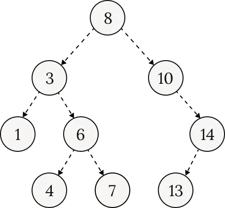
B-Tree takes the core idea and tweaks it a bit. What if we can have more than two children? Yes, that is B-Tree. The number of children is configurable, commonly referred to as degree (or order) in academic literature. We could consider binary search tree as a special case of B-Tree with degree 2. We say that B-Tree has higher fanout (the number of children a node can have) than binary search tree.

Terminology and invariants

To establish a shared vocabulary, here are some terms that I will mention throughout this blog post:

• B-Tree degree k: this number determines the fanout of the tree.
• As we said above, B-Tree only stores values at the leaf nodes. We distinguish nodes into 3 types:
1. Root node: this has no parents and is at the top of the tree.
2. Leaf nodes: these are the bottom layer nodes that have no child nodes. This is where we store values.
3. Internal nodes: these are nodes in between, connecting the root node to leaf nodes. They only store keys to separate the key space into different ranges. We call them separator keys. These nodes serve as guide posts to locate the correct leaf node that holds your key.

The design of B-Tree has a few invariants. Remember these, because they play a big role in how the data structure operates, as well as choosing design trade-offs.

1. Given a tree with degree k, a node (except the root node) must have at least k children and at most 2k children. In another word, a node must always be at least half full.
2. The keys inside each node must be ordered. This is not a strict requirement, but it’s beneficial to maintain a sorted order. Most real implementations do this.

Basic operations

Let’s look through some basic operations that B-Tree support: lookup, insert and delete.

Lookup

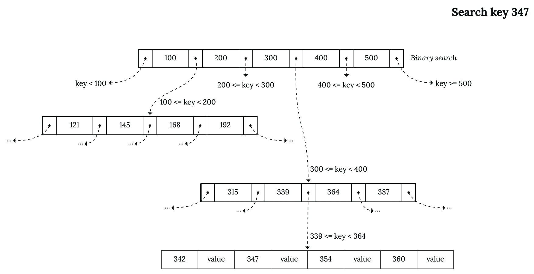
B-Tree can perform single key lookup (key = 42) or range scan (30 < key < 40). For single key lookup, the process is comparable to binary search tree. This description outlines the algorithm’s implementation:

1. Start at the root node.
2. Choose the correct child that contains your target key by comparing it with the separator keys. Since the separator keys are sorted, we can perform binary search on them.
3. Repeat step 2 to traverse down the tree.
4. If you reach a leaf node and it contains your target key, the lookup ends. If the leaf node doesn’t contain your target key, or you can’t find the leaf node (there’s no correct range in the internal nodes), it means your key does not exist in the data structure, and the lookup ends.

Let’s look at an illustration of the lookup process:

Range scans start off by looking up the lower bound value. Once we found the lower bound, start scanning the sibling keys. Some B-Tree variants have pointers between sibling nodes, which can speed up the scanning phase.

Insert

Since B-Tree is an ordered data structure, insertion needs to search for the correct slot. After we find the place, we insert the new value into the leaf page.

But, there’s a catch. Each node has a capacity of 2k keys, where k is the degree of the B-Tree. If the leaf node is full, we say that the node is overflowed. Two common approaches to dealing with this:

1. Split the overflowed node: The overflowed node is split into two nodes. Choosing the split point is a problem on its own, but the most common way is to split in the middle. After that, a new separator key is added to the parent node to point to the newly split node. If the parent node is again overflowed, repeat the split process. The split process can cascade upward from the leaf all the way to the root. This is the way that B-Tree grows in height.

2. Redistribute the keys: The keys from the overflowed node are redistributed to sibling nodes. Then, the parent node is updated to reflect the new changes.

Delete

Same as insertion, you first lookup the key then delete it. Simple right? Not so fast. Each node in B-Tree must include at least k children, where k is the degree of the B-Tree. If the node has fewer children, we say that the node is underflowed. Two common ways to solve this:

1. Redistribute the keys: You can steal keys from sibling nodes. After that, update the parent node to adjust for the new key ranges.

2. Merge with sibling nodes: If there is enough space, two nodes can merge into one. After the merge, there will be one less child, and the parent node must be updated to reflect this. This in turn could cause the parent node to underflow, and again, you can choose to redistribute or merge. The merge process can cascade up to the root. When two last children of the root is merge, the root is removed and the newly merged node becomes the root. This is the way that B-Tree shrinks in height.