Part 4

Optimizations

We can apply a number of optimizations on the baseline design of B-Tree, each with different trade-offs. They aim to provide more compact tree structure, better tree navigation or optimize cache utilization.

Sibling pointers

The name is self-explanatory: adding pointers to the left or right sibling to each node. Effectively, each level will become a linked list (or even a doubly linked list). This helps us quickly traverse the tree, which is useful during range scans. This technique is applied in many variations, both B+ Tree and B Link Tree as, we discussed previously.

Key normalization

This technique encodes keys into a binary string. The encoding scheme must preserve the key sorted order and comparison result. In another word, if A is greater than B, then the normalization of A is also greater than the normalization of B, and vice versa.

Key normalization improves overall performance since binary strings are faster to compare (we basically compare integers). A simple memcmp is all we need in all cases. But the true power of this technique is that binary strings are extremely flexible. Normalized keys are essentially strings of bytes, or strings of wider integers that can be easily concatenated, inverted, and truncated. This optimization unlocks a whole set of other optimizations: prefix compression and suffix truncation, which we will discuss later.

However, there are several drawbacks:

1. The normalized key tends to be bigger than the original key.
2. We cannot recover the original key from the normalized one. This affects cases where the original key is required, for example, PostgreSQL index-only scans. To alleviate this, implementations can apply normalization only on internal nodes. We don’t need their original values, we just need to perform comparisons.

Prefix compression

Consider this sorted sequence of keys inside a node:

Notice the common prefix? How about we only store it once? That’s the exact idea of prefix compression. It can significantly reduce the key size, which leads to more keys in internal nodes. And as we mentioned times and times before, higher fanout means faster B-Tree. Also, comparisons when searching don’t need to consider the prefix part.

The sorted nature of B-Tree enables this optimization. Since keys are ordered, neighbor keys are similar. In fact, they can be equal in the first few leading bytes, or even all bytes in case they are duplicated.

It’s possible to perform prefix compression without key normalization. But it would require a fair deal of bookeeping, even if they were applied only to entire key fields rather than to individual bytes. With key normalization, the implementation is straightforward, since all keys are just binary strings.

In the context of database indexes, prefix compression effects can be significant in certain cases. A typical multi-column index, especially with leading fields as foreign keys, might look like this:

Foreign keys increase the chance of encountering duplicate values. In the above example (though contrived), suffix compression can easily reduce the node size by a third. The trade-off is the added complexity and runtime overhead (original keys must be recreated on every operation). Sometimes, it’s not worth it if the tree doesn’t have that many duplicated keys.

Suffix truncation

Imagine we have a leaf node like this and we need to split it due to a new insert. Let say we split right in the middle. What should the separator key be?

The simplest solution is to choose the lowest value from the right node, Jake. But can we do better? Remember, the only function of separator keys is to divide the key space into two halves. One is strictly smaller than it, and the other one is greater or equal to it. We can choose any value, as long as it does its job.

In this case, J is the optimal choice. Part of the original key Jake gets truncated, hence the name suffix truncation.

If performing suffix truncation on arbitrary bytes like the above example is complex, you can apply it to the whole index field. Let’s bring back the customer_addresses table example.

If we split right in the middle, we can choose (Viet Nam, -∞) as the separator key. The negative infinity can be compactly represented to save bytes, similar to how databases represent NULL values. These negative infinity can also make comparisons faster since we can add a fast path specifically for them.

Similar to prefix compression, this technique aims to reduce the key size and leads to higher fanout. A B-Tree implementation with suffix truncation is sometimes said to be a “prefix B-Tree”. Key normalization greatly simplifies the implementation and increases the effectiveness, as we only have to deal with binary strings as keys.

That said, suffix truncation has one disadvantage. It can’t be applied to leaf nodes, just internal nodes. For the same reason in prefix compression, it’s not possible to recover the original keys. The internal nodes only make up about 1% of the total tree size, Therefore, the size reduction is often not noticeable.

Poor man’s normalized keys

So far, we mentioned optimizations applied to the key level. Let’s zoom out a little bit and look at B-Tree nodes. As we mentioned in Part 2, B-Tree node with variable length keys is commonly implemented as slotted page.

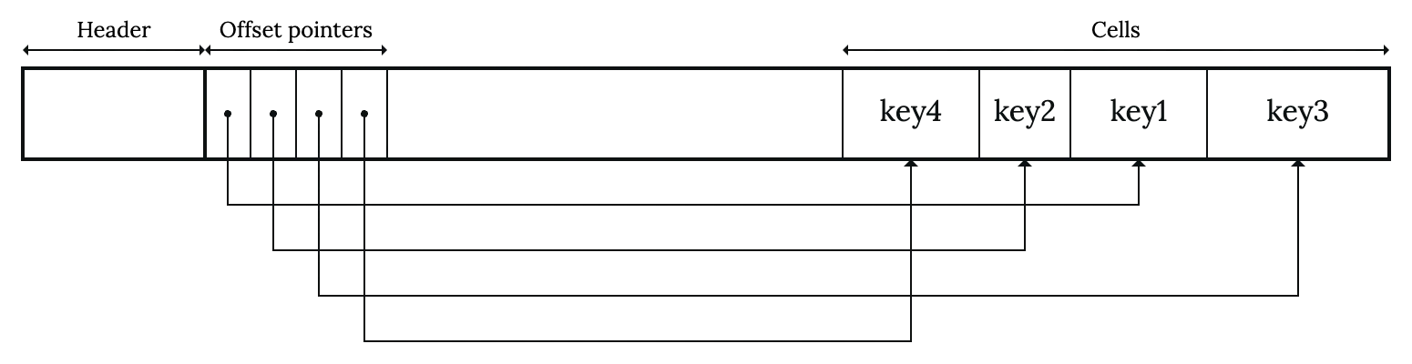
This scheme incurs some extra cost of memory accesses when searching for keys. Each jump during binary search will require two memory accesses: one for the offset pointer and one for the key content. For instance, if our node has 16 keys, we will need at most 10 accesses.

One trick is to store a few leading bytes of the key along with the offset pointer, basically making it “fat”. Let’s consider this example when we search for avocado key:

With 3 leading bytes, we can confidently say that the key does not exist without ever touching the actual keys. This is because those tiny bits of the original keys are enough to distinguish them. This fixed-size prefix is typically called a poor man’s normalized key in literature.

Nonetheless, this technique only works well if prefix compression presents. With common prefix truncated away, even a small poor man key (2 or 4 bytes) is enough to avoid some memory accesses. Otherwise, even a large poor man key might not be effective, especially in the leaf nodes, where keys are highly similar.